Kimchi is our new trustless zkSNARK that is based on the PLONK proof system and the Bulletproofs commitment scheme. The goal of this post is to relieve the symptoms produced after reading the former paper. After all, its carefully chosen acronym (Permutations over Lagrange-bases for Oecumenical Noninteractive arguments of Knowledge) is far from being just a funny coincidence: let us try to convert a bottle of plonk into this glass of silky wine, and cheers!

Kimchi

Usually, one would need some napa cabbage, salt and spices in order to cook homemade kimchi. At O(1) Labs, our Kimchi recipe is slightly different: instead of the above main ingredients, we will use these three Arguments.

• Custom gates: these are our spices to taste. Different configurations (flavours) will accompany different kimchi dishes. A bit more formally, depending on the type of computation we want to have proofs for, we will choose different custom gates to create our circuit.
• Permutation: just like napa cabbage, this is the ingredient that binds the flavours of a kimchi dish together, it makes kimchi a dish instead of just some spare components that do not talk to each other. More formally, the permutation argument performs the wiring between gates (the connections from/to inputs/outputs), representing copy constraints between cells in the execution trace.
• Lookup tables: the pinch of salt that is not really needed, but makes the result stand out. We can use lookup tables for efficiency reasons. Some public information can be stored by both parties (prover and verifier), instead of wired in the circuit, such as boolean functions.

All of these arguments are translated into equations that must hold for a correct witness for the full relation. Equivalently, this is to say that a number of expressions need to evaluate to zero on a certain set of numbers. Prior to cooking kimchi, we should make sure we know the procedures involved. So there are two problems to tackle here:

1. Roots-check: making sure the ingredients pass some quality test, or formally to check that an equation evaluates to zero on a set of numbers.
2. Aggregate: checking all ingredients, the above condition must hold for every single equation.

In the following, we will be making use of the notation $\mathbb{F}$ that refers to a finite field. You can think of these as mathematical structures of elements that behave like a clock. This means, that the largest element in the field wraps back into the smallest element (in the same way that 12am corresponds to 00:00). The nice property about these fields that we care about is the fact that numbers within these fields cannot grow ad infinitum, they are always kept within a range (called the order of the field). And still, algebra will hold (we call this modular algebra). Just a subtlety, the order of finite fields must be either a prime number or a power of a prime number. So get your thirteen-hours timer and let’s cook!

Roots-check

For the first problem, given a polynomial $p(X)$ of degree $d$, we are asking to check that $p(x)=0$ for all elements $x$ in a set $S$ (a collection of numbers). Of course, one could manually evaluate each of the elements in the set and make sure of the above claim. But that would take so long (i.e. it wouldn’t be succinct). Instead, we want to check it all at once. And a great way to do it is by using a vanishing polynomial. Such a polynomial $v_S(X)$ will be nothing else than the smallest polynomial that vanishes on $S$. That means, it is exactly defined as the degree $|S|$ polynomial formed by the product of the monomials:

$$v_S(X) = \prod_{s\in S} (X-s)$$

And why is this so advantageous? Well, first we need to make a key observation. Since the vanishing polynomial equals zero on every $x\in S$, and it is the smallest such polynomial (recall it has the smallest possible degree so that this property holds), if our initial polynomial $p(X)$ evaluates to zero on $S$, then it must be the case that $p(X)$ is a multiple of the vanishing polynomial $v_S(X)$. But what does this mean in practice? By polynomial division, it simply means there exists a quotient polynomial of degree $d-|S|$ such that:

$$q(X) := \frac{p(X)}{v_S(X)}$$

And still, where’s the hype? If you can provide such a quotient polynomial, one could easily check that if $q(a) = p(a) / v_S(a)$ for a random number $a\in\mathbb{F}$ \ $S$ (recall you will check in a point $a$ in the field but out of the set, otherwise you would get a $0/0$), then with very high probability that would mean that actually $p(X) = q(X) \cdot v_S(X)$, meaning that $p(X)$ vanishes on the whole set $S$, with just one point!

Let’s take a deeper look into the “magic” going on here. First, what do we mean by high probability? Is this even good enough? And the answer to this question is: as good as you want it to be.

First we analyse the math in this check. If the polynomial form of $p(X) = q(X) \cdot v_S(X)$ actually holds, then of course for any possible $a\in\mathbb{F}$ \ $S$ the check $p(a) =_? q(a) \cdot v_S(a)$ will hold. But is there any unlucky instantiation of the point $a$ such that $p(a) = q(a) \cdot v_S(a)$ but $p(X) \neq q(X) \cdot v_S(X)$? And the answer is, yes, there are, BUT not many. But how many? How unlikely is this? You already know the answer to this: Schwartz-Zippel. Recalling this lemma:

Given two different polynomials $f(X)$ and $g(X)$ of degree $d$, they can at most intersect (i.e. coincide) in $d$ points. Or what’s equivalent, let $h(X) := f(X) - g(X)$, the polynomial $h(X)$ can only evaluate to $0$ in at most $d$ points (its roots).

Thus, if we interchange $p(X) \rightarrow f(X)$ and $q(X)\cdot v_S(X) \rightarrow g(X)$, both of degree $d$, there are at most $\frac{d}{|\mathbb{F}- S|}$ unlucky points of $a$ that could trick you into thinking that $p(X)$ was a multiple of the vanishing polynomial (and thus being equal to zero on all of $S$). So, how can you make this error probability negligible? By having a field size that is big enough (the formal definition says that the inverse of its size should decrease faster than any polynomial expression). Since we are working with fields of size $2^{255}$, we are safe on this side!

Second, is this really faster than checking that $p(x)=0$ for all $x\in S$ ? At the end of the day, it seems like we need to evaluate $v_S(a)$, and since this is a degree $|S|$ polynomial it looks like we are still performing about the same order of computations. But here comes mathematics to the rescue again. In practice, we want to define this set $S$ to have a nice structure that allows us to perform some computations more efficiently than with arbitrary sets of numbers. Indeed, this set will normally be a multiplicative group (normally represented as $\mathbb{G}$ or $\mathbb{H}$), because in such groups the vanishing polynomial $v_\mathbb{G}(X):=\prod_{\omega\in\mathbb{G}}(X-\omega)$ has an efficient representation $v_\mathbb{G}(X)=X^{|\mathbb{G}|}-1$, which is much faster to evaluate than the above product.

Third, we may want to understand what happens with the evaluation of $p(a)$ instead. Since this is a degree $d ≥ |\mathbb{G}|$, it may look like this will take a lot of effort as well. But here’s where cryptography comes into play: various reasons why the verifier will never get to evaluate the actual polynomial by themselves. One, if the verifier had access to the full polynomial $p(X)$, then the prover should have sent it along with the proof, which would require $d+1$ coefficients to be represented (and this is no longer succinct for a SNARK). Two, this polynomial could carry some secret information, and if the verifier could recompute evaluations of it, they could learn some private data by evaluating on specific points. So instead, these evaluations will be a “mental game” thanks to polynomial commitments and proofs of evaluation sent by the prover (for whom a computation in the order of $d$ is not only acceptable, but necessary). The actual proof length will depend heavily on the type of polynomial commitments we are using. For example, in Kate-like commitments, committing to a polynomial takes a constant number of group elements (normally one), whereas in Bulletproofs it is logarithmic. But in any case this will be shorter than sending $O(d)$ elements.

Aggregate

So far we have seen how to check that a polynomial equals zero on all of $\mathbb{G}$, with just a single point. This is somehow an aggregation per se. But we are left to analyse how we can prove such a thing, for many polynomials. Altogether, if they hold, this will mean that the polynomials encode a correct witness and the relation would be satisfied. These checks can be performed one by one (checking that each of the quotients are indeed correct), or using an efficient aggregation mechanism and checking only one longer equation at once.

So what is the simplest way one could think of to perform this one-time check? Perhaps one could come up with the idea of adding up all of the equations $p_0(X),…,p_n(X)$ into a longer one $\sum_{i=0}^{n} p_i(X)$. But by doing this, we may be cancelling out terms and we could get an incorrect statement.

So instead, we can multiply each term in the sum by a random number. The reason why this trick works is the independence between random numbers. That is, if two different polynomials $f(X)$ and $g(X)$ are both equal to zero on a given $X=x$, then with very high probability the same $x$ will be a root of the random combination $\alpha\cdot f(x) + \beta\cdot g(x) = 0$. If applied to the whole statement, we could transform the $n$ equations into a single equation, $$\bigwedge_{i_n} p_i(X) =?\ 0 \iff_{w.h.p.} \sum_{i=0}^{n} \rho_i \cdot p_i(X) =?\ 0$$

This sounds great so far. But we are forgetting about an important part of proof systems which is proof length. For the above claim to be sound, the random values used for aggregation should be verifier-chosen, or at least prover-independent. So if the verifier had to communicate with the prover to inform about the random values being used, we would get an overhead of $n$ field elements.

Instead, we take advantage of another technique that is called powers-of-alpha. Here, we make the assumption that powers of a random value $\alpha^i$ are indistinguishable from actual random values $\rho_i$. Then, we can twist the above claim to use only one random element $\alpha$ to be agreed with the prover as:

$$\bigwedge_{i_n} p_i(X) =?\ 0 \iff_{w.h.p.} \sum_{i=0}^{n} \alpha^i \cdot p_i(X) =?\ 0$$

Gates

In the previous section we saw how we can prove that certain equations hold for a given set of numbers very efficiently. What’s left to understand is the motivation behind these techniques. Why is it so important that we can perform these operations and what do these equations represent in the real world?

But first, let’s recall the table that summarizes some important notation that will be used extensively:

One of the first ideas that we must grasp is the notion of a circuit. A circuit can be thought of as a set of gates with wires connecting them. The simplest type of circuit that one could think of is a boolean circuit. Boolean circuits only have binary values: $1$ and $0$, true and false. From a very high level, boolean circuits are like an intricate network of pipes, and the values could be seen as water or no water. Then, gates will be like stopcocks, making water flow or not between the pipes. This video is a cool representation of this idea. Then, each of these behaviours will represent a gate (i.e. logic gates). One can have circuits that can perform more operations, for instance arithmetic circuits. Here, the type of gates available will be arithmetic operations (additions and multiplications) and wires could have numeric values and we could perform any arbitrary computation.

If we spin the loop a bit more, we could come up with a single Generic gate that could represent any arithmetic operation at once. This thoughtful type of gate is the one gate whose concatenation is used in Plonk to describe any relation. Apart from its wires, these gates are tied to an array of coefficients that help describe the functionality. But the problem with this gate is that it takes a large set of them to represent any meaningful function. So instead, recent Plonk-like proof systems have appeared which use custom gates to represent repeatedly used functionalities more efficiently than as a series of generic gates connected to each other. Kimchi is one of these protocols. Currently, we give support to specific gates for the Poseidon hash function, the CompleteAdd operation for curve points, VarBaseMul for variable base multiplication, EndoMulScalar for endomorphism variable base scalar multiplication, and the ChaCha encryption primitive.

The circuit structure is known ahead of time, as this is part of the public information that is shared with the verifier. What is secret is what we call the witness of the relation, which is the correct instantiation of the inputs and wires of the circuit satisfying all of the checks. This means the verifier knows what type of gate appears in each part of the circuit, and the coefficients that are attached to each of them.

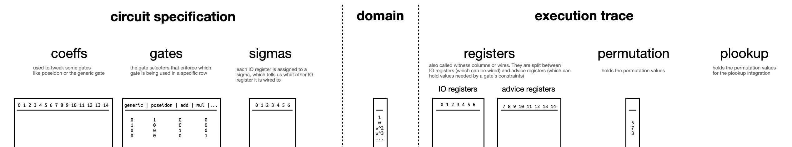
Gates are laid out as rows in a matrix with as many columns as desired (Plonk needs 3, whereas Kimchi currently uses 15). The execution trace refers to the state of all the wires throughout the circuit, upon instantiation of the witness. It will be represented as a table where the rows correspond to each gate and the columns refer to the actual wires of the gate (a.k.a. input and output registers) and some auxiliary values needed for the computation (a.k.a. advice registers). The current implementation of Kimchi considers a total of 15 columns with the first 7 columns corresponding to I/O registers. The permutation argument acts on the I/O registers (meaning, it will check that the cells in the first 7 columns of the execution trace will be copied correctly to their destination cells). For this reason, these checks are also known as copy constraints.

Let the 3 Plonk columns witnesses be $w_L, w_R$ and $w_O$, referring to left, right and output. Together with coefficients $c_L, c_R, c_O, c_M, c_S$ for left, right, output, multiplication and scalar, one can express generic arithmetic operations as $0 = c_L \cdot w_L + c_R \cdot w_R + c_O \cdot w_O + c_M \cdot w_L \cdot w_R + c_S$.

Coefficients act as binary selectors, except for the scalar coefficient that can be any constant. For example, additions can be represented by toggling off the multiplication selector $c_M$.

Going back to the main motivation of the scheme, recall that we wanted to check that certain equations hold in a given set of numbers. Here’s where this claim starts to make sense. The total number of rows in the execution trace will give us a domain. That is, we define a mapping between each of the row indices of the execution trace and the elements of a multiplicative group $\mathbb{G}$ with as many elements as rows in the table. Two things to note here. First, if no such group exists we can pad with zeroes. Second, any multiplicative group has a generator $g$ whose powers generate the whole group. Then we can assign to each row a power of $g$. Why do we want to do this? Because this will be the set over which we want to check our equations: we can transform a claim about the elements of a group to a claim like “these properties hold for each of the rows of this table”. Interesting, right?